Deutsch’s algorithm
Deutsch’s algorithm will be our first quantum algorithm to look into. As will be the style throughout the documentation, we will try to keep the mathematics to minimum and focus on the implementation. This doesn’t mean that we won’t try to understand why and how the algorithm works but we will seek to only use the mathematics necessary to get us to our goal. If it is your wish to study the algorithm in depth, references are given at the end of the section.
Here is how this section is organized: first, we will we will set up the problem with all the information necessary to understand the problem we are trying to solve. Then we will state the problem and comment on it. Afterwards we shall present a classical solution to the problem and comment on the solution. Following the classical solution we will present a quantum solution. Then we shall close with some concluding remarks.
Introduction
Imagine the following: you are given a function \(f:\mathbb{B} \to \mathbb{B}\) where \(\mathbb{B}=\{0, 1\}\). So this function takes zero or one and returns zero or one.
What are the possible input/output combinations of this function?
- First combination: \(f_{0}(0) \to 1\) and \(f_{0}(1) \to 1\).
- Second combination: \(f_{1}(0) \to 0\) and \(f_{1}(1) \to 1\).
- Third combination: \(f_{2}(0) \to 1\) and \(f_{2}(1) \to 0\).
- Fourth combination: \(f_{3}(0) \to 0\) and \(f_{3}(1) \to 0\).
Notice that for the first and the fourth combinations, the output doesn’t change irrespective of the input. The output is constant; hence the function is said to be constant in both combinations. The second and the third combinations though are different: the number of zeros in the output is the same as the number of ones. There is a balance in the output; hence we call it balanced in both combinations.
Balanced and constant functions
A function \(f:\mathbb{B} \to \mathbb{B}\) is said to be constant if \(f(0)=f(1)\). It is said to be balanced if \(f(0) \neq f(1)\).
There are lots of interesting questions we can ask about this function (yes, actually a lot). But here is one we are going to try to solve: suppose we are given one of the four combinations randomly. Without being told which one or being allowed to look inside, we are asked if it is balanced or constant. This is called Deutsch’s problem after David Deutsch who first proposed a quantum solution to this problem in 1985 (and mind you, his first solution worked only half the time). When we are given a function which implementation we don’t know, we call it a black box or more formally an oracle.
Deutsch’s problem
Let \(f:\mathbb{B} \to \mathbb{B}\) be an oracle. Is \(f\) balanced or constant?
One remark though, however obvious, is that we are going to need to call the oracle and pass it our input(s). Note that nothing is said about reading the output. Read on and find out why.
Note
Throughout the section, we are going to assume that we are given combinations as oracles of the form \(f_{i}(n)\) for \(i \in \{0, 1, 2, 3\}\) and \(n \in \mathbb{B}\).
Classical solution
So we are given the oracle, now we need to find out if it is balanced or constant. As programmers, part our business is finding out how to solve problems efficiently. Many things may go into the final solution but right now we do know that we would like to reduce the number of times we call the oracle. The more we call it the longer it will take to make our decision of whether we have a balanced or a constant oracle.
We can visualize the classical algorithm running as shown below.
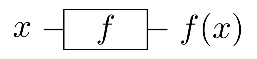
Fig. 1 Classical oracle executing the function \(f\).
So how many times exactly do we need to call the oracle here?
If we call the oracle passing it \(0\), the first combination will return \(1\). But the third combination will also return \(1\). Also, the second combination will return \(0\) when given \(0\) as input. We cannot hope to know if the oracle is balanced or constant by passing it \(0\) alone. The same argument applies when \(1\) is given as input.
But note that if we call the oracle with \(0\) then with \(1\), we can make some progress. If \(f(0)\) and \(f(1)\) are equal then we know the oracle is constant by definition. The same argument can be used by definition of a balanced function.
Therefore we need to call the oracle once for \(f(0)\) and once for \(f(1)\) to solve the problem. Two calls to the oracle are necessary (we can’t make a decision with only one call) and sufficient (we learn nothing new by a third call).
Here is the classical code that solves Deutsch’s problem.
You can find it in the deutsch folder in the algorithms repository at the Classical and Quantum Algorithms in Avalon.
import io
import oracles.classical


def __main__ = (val args : [string]) -> void:
    -- step 1 : call the oracle with 0
    val left = Oracle.f0(0b0)

    -- step 2 : call the oracle again but with 1
    val right = Oracle.f0(0b1)

    -- step 3 : compare both results to determine if the oracle is constant or balanced
    if left == right:
        Io.println("The oracle contains a constant function.")
    else:
        Io.println("The oracle contains a balanced function.")

    -- we are done
    return
Notice that we are calling the oracle twice, first in step 1 then in step 2. Therefore, any algorithm that allows us to solve the exact same problem in less than two calls (that is in one call) is better than the current classical algorithm. And coming right next up is that solution, first due to David Deutsch.
Quantum solution
Quantum algorithms are a bit harder to figure out and harder to reason about concerning their correctness. But we will do that here at the expense of explaining the oracles.
If you read the code for classical oracles, they are not hard to understand. But it is not immediately obvious how they got translated to quantum oracles. No matter, it is not our objective to construct the oracles, you are not supposed to peek into them anyway. So we are going to focus on the algorithm itself.
Classical oracle to quantum oracle
To get started, we need to transform the way the classical oracle is called into a flow the quantum algorithm can work with. We can’t use the flow in Fig. 1 because it is not reversible. So we need to build an equivalent flow that has the same effect but runnable on a quantum computer.
To make our oracles reversible, we use the following scheme, dubbing it XOR encoding of boolean functions.
XOR encoding of boolean functions
So we have transformed our classical function into a new function that is equivalent to it but with two important properties:
- The function \(U_f:\mathbb{B}^{n+1} \to \mathbb{B}\) is reversible.
- The original function \(f(x_1, x_2, \ldots, x_n):\mathbb{B}^n \to \mathbb{B}\) ouput can be recovered by taking \(y \oplus f(x_1, x_2, \ldots, x_n) \oplus y\).
The two properties above of the function \(U_f:\mathbb{B}^{n+1} \to \mathbb{B}\) mean that it is executable on a quantum computer and from the answer it provides we are able to recover the original answer the classical function would have given.
As mentioned above, we won’t see how to build oracles from \(U_f:\mathbb{B}^{n+1} \to \mathbb{B}\) but it is a good exercise if you want to try it. Neither are we going to actually find the output. We are going to do the following though:
- See how to use the oracles from \(U_f:\mathbb{B}^{n+1} \to \mathbb{B}\) in the algorithm.
- Understand how the algorithm solves Deutsch’s problem.
To begin, we are going to simplify the XOR encoding and limit \(f(x_1, x_2, \ldots, x_n):\mathbb{B}^n \to \mathbb{B}\) to \(f(x):\mathbb{B}^n \to \mathbb{B}\). This means that its encoding is given by \(U_f(x, y):\mathbb{B}^{2} \to \mathbb{B}\).
Then we are going to shift to the bracket notation in order to simplify calculations and make \(U_f(x, y):\mathbb{B}^{2} \to \mathbb{B}\) accept inputs of the form \(|x, y\rangle\). For our satisfaction, let us show that \(U_f(|x, y\rangle):\mathbb{B}^{2} \to \mathbb{B}\) is both reversible and \(f(x)\) can be recovered from it.
Let us first look at a circuit similar to the one in Fig. 1.
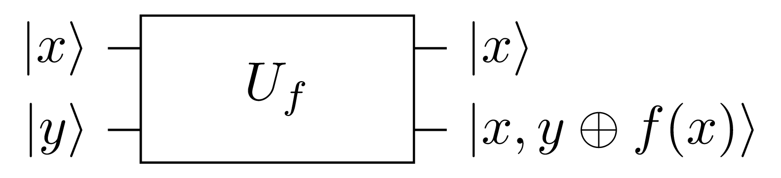
Fig. 2 Quantum oracle executing the function \(f\) using its encoding \(U_f(|x, y\rangle)=|x,y \oplus f(x)\rangle\).
The oracle is given two bits in the form \(|x, y\rangle\) and produces output of the form \(|x, y \oplus f(x)\rangle\). Looking at Fig. 2, we can see how the quantum oracle is truly quantum and at the same time can be used to get back the classical oracle.
- To get back the original oracle from the output, we ignore \(|x\rangle\) and XOR \(|y \oplus f(x)\rangle\) with \(|y\rangle\) resulting in \(|f(x)\rangle\) which is the result of the classical oracle.
- To prove that the quantum oracle is truly quantum and therefore must be reversible we only need to show that executing the oracle passing it its own output gives back the original input. To show that, let \(z = y \oplus f(x)\). Thus the new input is \(|x, z\rangle\). Giving that input to the oracle, the expected output is \(|x, z \oplus f(x)\rangle\). This output is equivalent to \(|x, (y \oplus f(x)) \oplus f(x)\rangle\). Rearranging, we get \(|x, y \oplus (f(x) \oplus f(x))\rangle\). And finally eliminating \(f(x)\) due to XOR, we get as final output \(|x, y\rangle\). And with that we have the original input! Therefore the quantum oracle is reversible.
Deutsch’s algorithm
We are ready to tackle the quantum algorithm. We won’t discuss how to derive it and will limit ourselves to understanding how it works. Why it works is another matter that is not presented and you are encouraged to read references given at the end of this section.
We present a circuit description of the algorithm from which we shall derive the final program.
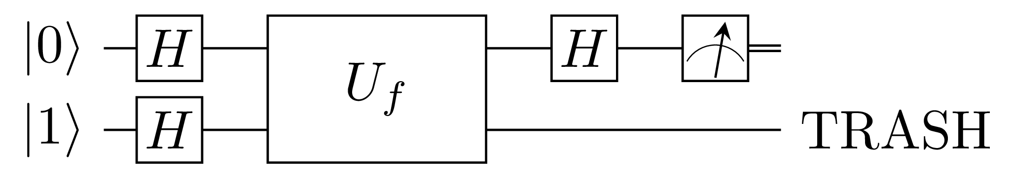
Fig. 3 Deutsch’s algorithm as the quantum solution to Deutsch’s problem.
Using Fig. 3 as reference, we are going to analyze what the algorithm does and how we find out if the oracle is balanced or constant from its output.